Analytical Solution for a 1D equilibrium interface
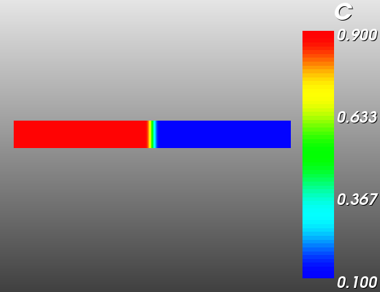
Composition for 2D simulation domain.
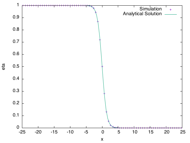
Order parameter along .
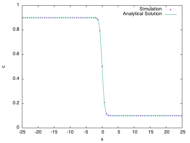
Composition along .
In the KKS model, an analytical solution exists for the order parameter and composition through a 1D equilibrium interface:
where we use the switching function , the gradient energy coefficient and the barrier function height . (Note that there is a typo in Eq. (49) of Kim et al. (1999), should be in the denominator of the argument to the function, not .) In the following example, we equilibrate a flat interface between a solid phase (, , ) and a liquid phase (, , ) in a 2D simulation. The vector postprocessor LineValueSampler is used to obtain the values of and along , the results are output to a CSV file, and plotted together with the 1D analytical solution. (We will use no-flux boundary conditions, so a boundary conditions block is not required in the input file.)
#
# KKS simple example in the split form
#

[Mesh<<<{"href": "../../../syntax/Mesh/index.html"}>>>]
  type = GeneratedMesh
  dim = 2
  nx = 150
  ny = 15
  nz = 0
  xmin = -25
  xmax = 25
  ymin = -2.5
  ymax = 2.5
  zmin = 0
  zmax = 0
  elem_type = QUAD4
[]

[AuxVariables<<<{"href": "../../../syntax/AuxVariables/index.html"}>>>]
  [./Fglobal]
    order<<<{"description": "Specifies the order of the FE shape function to use for this variable (additional orders not listed are allowed)"}>>> = CONSTANT
    family<<<{"description": "Specifies the family of FE shape functions to use for this variable"}>>> = MONOMIAL
  [../]
[]

[Variables<<<{"href": "../../../syntax/Variables/index.html"}>>>]
  # order parameter
  [./eta]
    order<<<{"description": "Specifies the order of the FE shape function to use for this variable (additional orders not listed are allowed)"}>>> = FIRST
    family<<<{"description": "Specifies the family of FE shape functions to use for this variable"}>>> = LAGRANGE
  [../]

  # solute concentration
  [./c]
    order<<<{"description": "Specifies the order of the FE shape function to use for this variable (additional orders not listed are allowed)"}>>> = FIRST
    family<<<{"description": "Specifies the family of FE shape functions to use for this variable"}>>> = LAGRANGE
  [../]

  # chemical potential
  [./w]
    order<<<{"description": "Specifies the order of the FE shape function to use for this variable (additional orders not listed are allowed)"}>>> = FIRST
    family<<<{"description": "Specifies the family of FE shape functions to use for this variable"}>>> = LAGRANGE
  [../]

  # Liquid phase solute concentration
  [./cl]
    order<<<{"description": "Specifies the order of the FE shape function to use for this variable (additional orders not listed are allowed)"}>>> = FIRST
    family<<<{"description": "Specifies the family of FE shape functions to use for this variable"}>>> = LAGRANGE
    initial_condition<<<{"description": "Specifies a constant initial condition for this variable"}>>> = 0.1
  [../]
  # Solid phase solute concentration
  [./cs]
    order<<<{"description": "Specifies the order of the FE shape function to use for this variable (additional orders not listed are allowed)"}>>> = FIRST
    family<<<{"description": "Specifies the family of FE shape functions to use for this variable"}>>> = LAGRANGE
    initial_condition<<<{"description": "Specifies a constant initial condition for this variable"}>>> = 0.9
  [../]
[]

[Functions<<<{"href": "../../../syntax/Functions/index.html"}>>>]
  [./ic_func_eta]
    type = ParsedFunction<<<{"description": "Function created by parsing a string", "href": "../../../source/functions/MooseParsedFunction.html"}>>>
    expression<<<{"description": "The user defined function."}>>> = '0.5*(1.0-tanh((x)/sqrt(2.0)))'
  [../]
  [./ic_func_c]
    type = ParsedFunction<<<{"description": "Function created by parsing a string", "href": "../../../source/functions/MooseParsedFunction.html"}>>>
    expression<<<{"description": "The user defined function."}>>> = '0.9*(0.5*(1.0-tanh(x/sqrt(2.0))))^3*(6*(0.5*(1.0-tanh(x/sqrt(2.0))))^2-15*(0.5*(1.0-tanh(x/sqrt(2.0))))+10)+0.1*(1-(0.5*(1.0-tanh(x/sqrt(2.0))))^3*(6*(0.5*(1.0-tanh(x/sqrt(2.0))))^2-15*(0.5*(1.0-tanh(x/sqrt(2.0))))+10))'
  [../]
[]

[ICs<<<{"href": "../../../syntax/ICs/index.html"}>>>]
  [./eta]
    variable<<<{"description": "The variable this initial condition is supposed to provide values for."}>>> = eta
    type = FunctionIC<<<{"description": "An initial condition that uses a normal function of x, y, z to produce values (and optionally gradients) for a field variable.", "href": "../../../source/ics/FunctionIC.html"}>>>
    function<<<{"description": "The initial condition function."}>>> = ic_func_eta
  [../]
  [./c]
    variable<<<{"description": "The variable this initial condition is supposed to provide values for."}>>> = c
    type = FunctionIC<<<{"description": "An initial condition that uses a normal function of x, y, z to produce values (and optionally gradients) for a field variable.", "href": "../../../source/ics/FunctionIC.html"}>>>
    function<<<{"description": "The initial condition function."}>>> = ic_func_c
  [../]
[]

[Materials<<<{"href": "../../../syntax/Materials/index.html"}>>>]
  # Free energy of the liquid
  [./fl]
    type = DerivativeParsedMaterial<<<{"description": "Parsed Function Material with automatic derivatives.", "href": "../../../source/materials/DerivativeParsedMaterial.html"}>>>
    property_name<<<{"description": "Name of the parsed material property"}>>> = fl
    coupled_variables<<<{"description": "Vector of variables used in the parsed function"}>>> = 'cl'
    expression<<<{"description": "Parsed function (see FParser) expression for the parsed material"}>>> = '(0.1-cl)^2'
  [../]

  # Free energy of the solid
  [./fs]
    type = DerivativeParsedMaterial<<<{"description": "Parsed Function Material with automatic derivatives.", "href": "../../../source/materials/DerivativeParsedMaterial.html"}>>>
    property_name<<<{"description": "Name of the parsed material property"}>>> = fs
    coupled_variables<<<{"description": "Vector of variables used in the parsed function"}>>> = 'cs'
    expression<<<{"description": "Parsed function (see FParser) expression for the parsed material"}>>> = '(0.9-cs)^2'
  [../]

  # h(eta)
  [./h_eta]
    type = SwitchingFunctionMaterial<<<{"description": "Helper material to provide $h(\\eta)$ and its derivative in one of two polynomial forms.\nSIMPLE: $3\\eta^2-2\\eta^3$\nHIGH: $\\eta^3(6\\eta^2-15\\eta+10)$", "href": "../../../source/materials/SwitchingFunctionMaterial.html"}>>>
    h_order<<<{"description": "Polynomial order of the switching function h(eta)"}>>> = HIGH
    eta<<<{"description": "Order parameter variable"}>>> = eta
  [../]

  # g(eta)
  [./g_eta]
    type = BarrierFunctionMaterial<<<{"description": "Helper material to provide $g(\\eta)$ and its derivative in a polynomial.\nSIMPLE: $\\eta^2(1-\\eta)^2$\nLOW: $\\eta(1-\\eta)$\nHIGH: $\\eta^2(1-\\eta^2)^2$", "href": "../../../source/materials/BarrierFunctionMaterial.html"}>>>
    g_order<<<{"description": "Polynomial order of the barrier function g(eta)"}>>> = SIMPLE
    eta<<<{"description": "Order parameter variable"}>>> = eta
  [../]

  # constant properties
  [./constants]
    type = GenericConstantMaterial<<<{"description": "Declares material properties based on names and values prescribed by input parameters.", "href": "../../../source/materials/GenericConstantMaterial.html"}>>>
    prop_names<<<{"description": "The names of the properties this material will have"}>>>  = 'M   L   eps_sq'
    prop_values<<<{"description": "The values associated with the named properties"}>>> = '0.7 0.7 1.0  '
  [../]
[]

[Kernels<<<{"href": "../../../syntax/Kernels/index.html"}>>>]
  active<<<{"description": "If specified only the blocks named will be visited and made active"}>>> = 'PhaseConc ChemPotSolute CHBulk ACBulkF ACBulkC ACInterface dcdt detadt ckernel'

  # enforce c = (1-h(eta))*cl + h(eta)*cs
  [./PhaseConc]
    type = KKSPhaseConcentration<<<{"description": "KKS model kernel to enforce the decomposition of concentration into phase concentration  $(1-h(\\eta))c_a + h(\\eta)c_b - c = 0$. The non-linear variable of this kernel is $c_b$.", "href": "../../../source/kernels/KKSPhaseConcentration.html"}>>>
    ca<<<{"description": "Phase a concentration"}>>>       = cl
    variable<<<{"description": "The name of the variable that this residual object operates on"}>>> = cs
    c<<<{"description": "Real concentration"}>>>        = c
    eta<<<{"description": "Phase a/b order parameter"}>>>      = eta
  [../]

  # enforce pointwise equality of chemical potentials
  [./ChemPotSolute]
    type = KKSPhaseChemicalPotential<<<{"description": "KKS model kernel to enforce the pointwise equality of phase chemical potentials $dF_a/dc_a = dF_b/dc_b$. The non-linear variable of this kernel is $c_a$.", "href": "../../../source/kernels/KKSPhaseChemicalPotential.html"}>>>
    variable<<<{"description": "The name of the variable that this residual object operates on"}>>> = cl
    cb<<<{"description": "Phase b concentration"}>>>       = cs
    fa_name<<<{"description": "Base name of the free energy function Fa (f_name in the corresponding derivative function material)"}>>>  = fl
    fb_name<<<{"description": "Base name of the free energy function Fb (f_name in the corresponding derivative function material)"}>>>  = fs
  [../]

  #
  # Cahn-Hilliard Equation
  #
  [./CHBulk]
    type = KKSSplitCHCRes<<<{"description": "KKS model kernel for the split Bulk Cahn-Hilliard term. This kernel operates on the physical concentration 'c' as the non-linear variable", "href": "../../../source/kernels/KKSSplitCHCRes.html"}>>>
    variable<<<{"description": "The name of the variable that this residual object operates on"}>>> = c
    ca<<<{"description": "phase concentration corresponding to the non-linear variable of this kernel"}>>>       = cl
    fa_name<<<{"description": "Base name of an arbitrary phase free energy function F (f_base in the corresponding KKSBaseMaterial)"}>>>  = fl
    w<<<{"description": "Chemical potential non-linear helper variable for the split solve"}>>>        = w
  [../]

  [./dcdt]
    type = CoupledTimeDerivative<<<{"description": "Time derivative Kernel that acts on a coupled variable. Weak form: $(\\psi_i, \\frac{\\partial v_h}{\\partial t})$.", "href": "../../../source/kernels/CoupledTimeDerivative.html"}>>>
    variable<<<{"description": "The name of the variable that this residual object operates on"}>>> = w
    v<<<{"description": "Coupled variable"}>>> = c
  [../]
  [./ckernel]
    type = SplitCHWRes<<<{"description": "Split formulation Cahn-Hilliard Kernel for the chemical potential variable with a scalar (isotropic) mobility", "href": "../../../source/kernels/SplitCHWRes.html"}>>>
    mob_name<<<{"description": "The mobility used with the kernel"}>>> = M
    variable<<<{"description": "The name of the variable that this residual object operates on"}>>> = w
  [../]

  #
  # Allen-Cahn Equation
  #
  [./ACBulkF]
    type = KKSACBulkF<<<{"description": "KKS model kernel (part 1 of 2) for the Bulk Allen-Cahn. This includes all terms NOT dependent on chemical potential.", "href": "../../../source/kernels/KKSACBulkF.html"}>>>
    variable<<<{"description": "The name of the variable that this residual object operates on"}>>> = eta
    fa_name<<<{"description": "Base name of the free energy function F (f_base in the corresponding KKSBaseMaterial)"}>>>  = fl
    fb_name<<<{"description": "Base name of the free energy function F (f_base in the corresponding KKSBaseMaterial)"}>>>  = fs
    w<<<{"description": "Double well height parameter"}>>>        = 1.0
    coupled_variables<<<{"description": "Vector of nonlinear variable arguments this object depends on"}>>> = 'cl cs'
  [../]
  [./ACBulkC]
    type = KKSACBulkC<<<{"description": "KKS model kernel (part 2 of 2) for the Bulk Allen-Cahn. This includes all terms dependent on chemical potential.", "href": "../../../source/kernels/KKSACBulkC.html"}>>>
    variable<<<{"description": "The name of the variable that this residual object operates on"}>>> = eta
    ca<<<{"description": "a-phase concentration"}>>>       = cl
    cb<<<{"description": "b-phase concentration"}>>>       = cs
    fa_name<<<{"description": "Base name of the free energy function F (f_base in the corresponding KKSBaseMaterial)"}>>>  = fl
  [../]
  [./ACInterface]
    type = ACInterface<<<{"description": "Gradient energy Allen-Cahn Kernel", "href": "../../../source/kernels/ACInterface.html"}>>>
    variable<<<{"description": "The name of the variable that this residual object operates on"}>>> = eta
    kappa_name<<<{"description": "The kappa used with the kernel"}>>> = eps_sq
  [../]
  [./detadt]
    type = TimeDerivative<<<{"description": "The time derivative operator with the weak form of $(\\psi_i, \\frac{\\partial u_h}{\\partial t})$.", "href": "../../../source/kernels/TimeDerivative.html"}>>>
    variable<<<{"description": "The name of the variable that this residual object operates on"}>>> = eta
  [../]
[]

[AuxKernels<<<{"href": "../../../syntax/AuxKernels/index.html"}>>>]
  [./GlobalFreeEnergy]
    variable<<<{"description": "The name of the variable that this object applies to"}>>> = Fglobal
    type = KKSGlobalFreeEnergy<<<{"description": "Total free energy in KKS system, including chemical, barrier and gradient terms", "href": "../../../source/auxkernels/KKSGlobalFreeEnergy.html"}>>>
    fa_name<<<{"description": "Base name of the free energy function F (f_name in the corresponding derivative function material)"}>>> = fl
    fb_name<<<{"description": "Base name of the free energy function F (f_name in the corresponding derivative function material)"}>>> = fs
    w<<<{"description": "Double well height parameter"}>>> = 1.0
  [../]
[]

[Executioner<<<{"href": "../../../syntax/Executioner/index.html"}>>>]
  type = Transient
  solve_type = 'PJFNK'

  petsc_options_iname = '-pc_type -sub_pc_type -sub_pc_factor_shift_type'
  petsc_options_value = 'asm      ilu          nonzero'

  l_max_its = 100
  nl_max_its = 100

  num_steps = 50
  dt = 0.1
[]

#
# Precondition using handcoded off-diagonal terms
#
[Preconditioning<<<{"href": "../../../syntax/Preconditioning/index.html"}>>>]
  [./full]
    type = SMP<<<{"description": "Single matrix preconditioner (SMP) builds a preconditioner using user defined off-diagonal parts of the Jacobian.", "href": "../../../source/preconditioners/SingleMatrixPreconditioner.html"}>>>
    full<<<{"description": "Set to true if you want the full set of couplings between variables simply for convenience so you don't have to set every off_diag_row and off_diag_column combination."}>>> = true
  [../]
[]

[VectorPostprocessors<<<{"href": "../../../syntax/VectorPostprocessors/index.html"}>>>]
  [./c]
    type =  LineValueSampler<<<{"description": "Samples variable(s) along a specified line", "href": "../../../source/vectorpostprocessors/LineValueSampler.html"}>>>
    start_point<<<{"description": "The beginning of the line"}>>> = '-25 0 0'
    end_point<<<{"description": "The ending of the line"}>>> = '25 0 0'
    variable<<<{"description": "The names of the variables that this VectorPostprocessor operates on"}>>> = c
    num_points<<<{"description": "The number of points to sample along the line"}>>> = 151
    sort_by<<<{"description": "What to sort the samples by"}>>> =  id
    execute_on<<<{"description": "The list of flag(s) indicating when this object should be executed. For a description of each flag, see https://mooseframework.inl.gov/source/interfaces/SetupInterface.html."}>>> = timestep_end
  [../]
  [./eta]
    type =  LineValueSampler<<<{"description": "Samples variable(s) along a specified line", "href": "../../../source/vectorpostprocessors/LineValueSampler.html"}>>>
    start_point<<<{"description": "The beginning of the line"}>>> = '-25 0 0'
    end_point<<<{"description": "The ending of the line"}>>> = '25 0 0'
    variable<<<{"description": "The names of the variables that this VectorPostprocessor operates on"}>>> = eta
    num_points<<<{"description": "The number of points to sample along the line"}>>> = 151
    sort_by<<<{"description": "What to sort the samples by"}>>> =  id
    execute_on<<<{"description": "The list of flag(s) indicating when this object should be executed. For a description of each flag, see https://mooseframework.inl.gov/source/interfaces/SetupInterface.html."}>>> = timestep_end
  [../]

[]

[Outputs<<<{"href": "../../../syntax/Outputs/index.html"}>>>]
  exodus<<<{"description": "Output the results using the default settings for Exodus output."}>>> = true
  [./csv]
    type = CSV<<<{"description": "Output for postprocessors, vector postprocessors, and scalar variables using comma seperated values (CSV).", "href": "../../../source/outputs/CSV.html"}>>>
    execute_on<<<{"description": "The list of flag(s) indicating when this object should be executed. For a description of each flag, see https://mooseframework.inl.gov/source/interfaces/SetupInterface.html."}>>> = final
  [../]
[]Verification against analytical solution
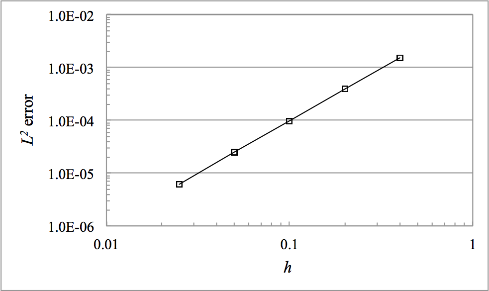
error for order parameter .
To perform a more quantitative comparison of the simulation results to the analytical solution, we will calculate the norm of the difference between the simulation result and the analytical solution. The norm is defined for this case as
where is the analytical solution, is the equilibrium solution from simulation, and is the domain. The norm can be obtained in the MOOSE framework using the ElementL2Error postprocessor. It can be shown from the properties of the finite element method that for the linear Lagrange elements used in the split formulation,
where is the characteristic element size (for 2D square elements, is the length of one side) and is a constant specific to the problem. Thus, as the mesh is refined, error should decrease (at least) quadratically with .
In performing this comparison between the analytical solution and simulation results, if a no-flux boundary condition is used in the simulation, the order parameter and composition profiles may shift slightly in the or direction, even if the analytical solution is used as an initial condition. This makes it difficult to compare to an analytical solution centered at . Therefore, we simulate the half of the domain and use a Dirichlet boundary condition of and at , which prevents the interface from moving. For the verification, the size of the domain was also reduced to lower the computational cost.
To verify that error decreases quadratically with , see the plot showing error versus for in this problem. As expected, on a log-log scale, the points are fit well by a straight line. The slope was determined to be 1.995, in good agreement with the expected value of 2.
#
# KKS simple example in the split form
#

[Mesh<<<{"href": "../../../syntax/Mesh/index.html"}>>>]
  type = GeneratedMesh
  dim = 2
  elem_type = QUAD4
  nx = 50
  ny = 2
  nz = 0
  xmin = 0
  xmax = 20
  ymin = 0
  ymax = 0.4
  zmin = 0
  zmax = 0
[]

[AuxVariables<<<{"href": "../../../syntax/AuxVariables/index.html"}>>>]
  [./Fglobal]
    order<<<{"description": "Specifies the order of the FE shape function to use for this variable (additional orders not listed are allowed)"}>>> = CONSTANT
    family<<<{"description": "Specifies the family of FE shape functions to use for this variable"}>>> = MONOMIAL
  [../]
[]

[Variables<<<{"href": "../../../syntax/Variables/index.html"}>>>]
  # order parameter
  [./eta]
    order<<<{"description": "Specifies the order of the FE shape function to use for this variable (additional orders not listed are allowed)"}>>> = FIRST
    family<<<{"description": "Specifies the family of FE shape functions to use for this variable"}>>> = LAGRANGE
  [../]

  # hydrogen concentration
  [./c]
    order<<<{"description": "Specifies the order of the FE shape function to use for this variable (additional orders not listed are allowed)"}>>> = FIRST
    family<<<{"description": "Specifies the family of FE shape functions to use for this variable"}>>> = LAGRANGE
  [../]

  # chemical potential
  [./w]
    order<<<{"description": "Specifies the order of the FE shape function to use for this variable (additional orders not listed are allowed)"}>>> = FIRST
    family<<<{"description": "Specifies the family of FE shape functions to use for this variable"}>>> = LAGRANGE
  [../]

  # Liquid phase solute concentration
  [./cl]
    order<<<{"description": "Specifies the order of the FE shape function to use for this variable (additional orders not listed are allowed)"}>>> = FIRST
    family<<<{"description": "Specifies the family of FE shape functions to use for this variable"}>>> = LAGRANGE
    initial_condition<<<{"description": "Specifies a constant initial condition for this variable"}>>> = 0.1
  [../]
  # Solid phase solute concentration
  [./cs]
    order<<<{"description": "Specifies the order of the FE shape function to use for this variable (additional orders not listed are allowed)"}>>> = FIRST
    family<<<{"description": "Specifies the family of FE shape functions to use for this variable"}>>> = LAGRANGE
    initial_condition<<<{"description": "Specifies a constant initial condition for this variable"}>>> = 0.9
  [../]
[]

[Functions<<<{"href": "../../../syntax/Functions/index.html"}>>>]
  [./ic_func_eta]
    type = ParsedFunction<<<{"description": "Function created by parsing a string", "href": "../../../source/functions/MooseParsedFunction.html"}>>>
    expression<<<{"description": "The user defined function."}>>> = 0.5*(1.0-tanh((x)/sqrt(2.0)))
  [../]
  [./ic_func_c]
    type = ParsedFunction<<<{"description": "Function created by parsing a string", "href": "../../../source/functions/MooseParsedFunction.html"}>>>
    expression<<<{"description": "The user defined function."}>>> = '0.9*(0.5*(1.0-tanh(x/sqrt(2.0))))^3*(6*(0.5*(1.0-tanh(x/sqrt(2.0))))^2-15*(0.5*(1.0-tanh(x/sqrt(2.0))))+10)+0.1*(1-(0.5*(1.0-tanh(x/sqrt(2.0))))^3*(6*(0.5*(1.0-tanh(x/sqrt(2.0))))^2-15*(0.5*(1.0-tanh(x/sqrt(2.0))))+10))'
  [../]
[]

[ICs<<<{"href": "../../../syntax/ICs/index.html"}>>>]
  [./eta]
    variable<<<{"description": "The variable this initial condition is supposed to provide values for."}>>> = eta
    type = FunctionIC<<<{"description": "An initial condition that uses a normal function of x, y, z to produce values (and optionally gradients) for a field variable.", "href": "../../../source/ics/FunctionIC.html"}>>>
    function<<<{"description": "The initial condition function."}>>> = ic_func_eta
  [../]
  [./c]
    variable<<<{"description": "The variable this initial condition is supposed to provide values for."}>>> = c
    type = FunctionIC<<<{"description": "An initial condition that uses a normal function of x, y, z to produce values (and optionally gradients) for a field variable.", "href": "../../../source/ics/FunctionIC.html"}>>>
    function<<<{"description": "The initial condition function."}>>> = ic_func_c
  [../]
[]

[BCs<<<{"href": "../../../syntax/BCs/index.html"}>>>]
  [./left_c]
    type = DirichletBC<<<{"description": "Imposes the essential boundary condition $u=g$, where $g$ is a constant, controllable value.", "href": "../../../source/bcs/DirichletBC.html"}>>>
    variable<<<{"description": "The name of the variable that this residual object operates on"}>>> = 'c'
    boundary<<<{"description": "The list of boundary IDs from the mesh where this object applies"}>>> = 'left'
    value<<<{"description": "Value of the BC"}>>> = 0.5
  [../]
  [./left_eta]
    type = DirichletBC<<<{"description": "Imposes the essential boundary condition $u=g$, where $g$ is a constant, controllable value.", "href": "../../../source/bcs/DirichletBC.html"}>>>
    variable<<<{"description": "The name of the variable that this residual object operates on"}>>> = 'eta'
    boundary<<<{"description": "The list of boundary IDs from the mesh where this object applies"}>>> = 'left'
    value<<<{"description": "Value of the BC"}>>> = 0.5
  [../]
[]

[Materials<<<{"href": "../../../syntax/Materials/index.html"}>>>]
  # Free energy of the liquid
  [./fl]
    type = DerivativeParsedMaterial<<<{"description": "Parsed Function Material with automatic derivatives.", "href": "../../../source/materials/DerivativeParsedMaterial.html"}>>>
    property_name<<<{"description": "Name of the parsed material property"}>>> = fl
    coupled_variables<<<{"description": "Vector of variables used in the parsed function"}>>> = 'cl'
    expression<<<{"description": "Parsed function (see FParser) expression for the parsed material"}>>> = '(0.1-cl)^2'
  [../]

  # Free energy of the solid
  [./fs]
    type = DerivativeParsedMaterial<<<{"description": "Parsed Function Material with automatic derivatives.", "href": "../../../source/materials/DerivativeParsedMaterial.html"}>>>
    property_name<<<{"description": "Name of the parsed material property"}>>> = fs
    coupled_variables<<<{"description": "Vector of variables used in the parsed function"}>>> = 'cs'
    expression<<<{"description": "Parsed function (see FParser) expression for the parsed material"}>>> = '(0.9-cs)^2'
  [../]

  # h(eta)
  [./h_eta]
    type = SwitchingFunctionMaterial<<<{"description": "Helper material to provide $h(\\eta)$ and its derivative in one of two polynomial forms.\nSIMPLE: $3\\eta^2-2\\eta^3$\nHIGH: $\\eta^3(6\\eta^2-15\\eta+10)$", "href": "../../../source/materials/SwitchingFunctionMaterial.html"}>>>
    h_order<<<{"description": "Polynomial order of the switching function h(eta)"}>>> = HIGH
    eta<<<{"description": "Order parameter variable"}>>> = eta
  [../]

  # g(eta)
  [./g_eta]
    type = BarrierFunctionMaterial<<<{"description": "Helper material to provide $g(\\eta)$ and its derivative in a polynomial.\nSIMPLE: $\\eta^2(1-\\eta)^2$\nLOW: $\\eta(1-\\eta)$\nHIGH: $\\eta^2(1-\\eta^2)^2$", "href": "../../../source/materials/BarrierFunctionMaterial.html"}>>>
    g_order<<<{"description": "Polynomial order of the barrier function g(eta)"}>>> = SIMPLE
    eta<<<{"description": "Order parameter variable"}>>> = eta
  [../]

  # constant properties
  [./constants]
    type = GenericConstantMaterial<<<{"description": "Declares material properties based on names and values prescribed by input parameters.", "href": "../../../source/materials/GenericConstantMaterial.html"}>>>
    prop_names<<<{"description": "The names of the properties this material will have"}>>>  = 'M   L   eps_sq'
    prop_values<<<{"description": "The values associated with the named properties"}>>> = '0.7 0.7 1.0  '
  [../]
[]

[Kernels<<<{"href": "../../../syntax/Kernels/index.html"}>>>]
  # enforce c = (1-h(eta))*cl + h(eta)*cs
  [./PhaseConc]
    type = KKSPhaseConcentration<<<{"description": "KKS model kernel to enforce the decomposition of concentration into phase concentration  $(1-h(\\eta))c_a + h(\\eta)c_b - c = 0$. The non-linear variable of this kernel is $c_b$.", "href": "../../../source/kernels/KKSPhaseConcentration.html"}>>>
    ca<<<{"description": "Phase a concentration"}>>>       = cl
    variable<<<{"description": "The name of the variable that this residual object operates on"}>>> = cs
    c<<<{"description": "Real concentration"}>>>        = c
    eta<<<{"description": "Phase a/b order parameter"}>>>      = eta
  [../]

  # enforce pointwise equality of chemical potentials
  [./ChemPotSolute]
    type = KKSPhaseChemicalPotential<<<{"description": "KKS model kernel to enforce the pointwise equality of phase chemical potentials $dF_a/dc_a = dF_b/dc_b$. The non-linear variable of this kernel is $c_a$.", "href": "../../../source/kernels/KKSPhaseChemicalPotential.html"}>>>
    variable<<<{"description": "The name of the variable that this residual object operates on"}>>> = cl
    cb<<<{"description": "Phase b concentration"}>>>       = cs
    fa_name<<<{"description": "Base name of the free energy function Fa (f_name in the corresponding derivative function material)"}>>>  = fl
    fb_name<<<{"description": "Base name of the free energy function Fb (f_name in the corresponding derivative function material)"}>>>  = fs
  [../]

  #
  # Cahn-Hilliard Equation
  #
  [./CHBulk]
    type = KKSSplitCHCRes<<<{"description": "KKS model kernel for the split Bulk Cahn-Hilliard term. This kernel operates on the physical concentration 'c' as the non-linear variable", "href": "../../../source/kernels/KKSSplitCHCRes.html"}>>>
    variable<<<{"description": "The name of the variable that this residual object operates on"}>>> = c
    ca<<<{"description": "phase concentration corresponding to the non-linear variable of this kernel"}>>>       = cl
    fa_name<<<{"description": "Base name of an arbitrary phase free energy function F (f_base in the corresponding KKSBaseMaterial)"}>>>  = fl
    w<<<{"description": "Chemical potential non-linear helper variable for the split solve"}>>>        = w
  [../]

  [./dcdt]
    type = CoupledTimeDerivative<<<{"description": "Time derivative Kernel that acts on a coupled variable. Weak form: $(\\psi_i, \\frac{\\partial v_h}{\\partial t})$.", "href": "../../../source/kernels/CoupledTimeDerivative.html"}>>>
    variable<<<{"description": "The name of the variable that this residual object operates on"}>>> = w
    v<<<{"description": "Coupled variable"}>>> = c
  [../]
  [./ckernel]
    type = SplitCHWRes<<<{"description": "Split formulation Cahn-Hilliard Kernel for the chemical potential variable with a scalar (isotropic) mobility", "href": "../../../source/kernels/SplitCHWRes.html"}>>>
    mob_name<<<{"description": "The mobility used with the kernel"}>>> = M
    variable<<<{"description": "The name of the variable that this residual object operates on"}>>> = w
  [../]

  #
  # Allen-Cahn Equation
  #
  [./ACBulkF]
    type = KKSACBulkF<<<{"description": "KKS model kernel (part 1 of 2) for the Bulk Allen-Cahn. This includes all terms NOT dependent on chemical potential.", "href": "../../../source/kernels/KKSACBulkF.html"}>>>
    variable<<<{"description": "The name of the variable that this residual object operates on"}>>> = eta
    fa_name<<<{"description": "Base name of the free energy function F (f_base in the corresponding KKSBaseMaterial)"}>>>  = fl
    fb_name<<<{"description": "Base name of the free energy function F (f_base in the corresponding KKSBaseMaterial)"}>>>  = fs
    w<<<{"description": "Double well height parameter"}>>>        = 1.0
    coupled_variables<<<{"description": "Vector of nonlinear variable arguments this object depends on"}>>> = 'cl cs'
  [../]
  [./ACBulkC]
    type = KKSACBulkC<<<{"description": "KKS model kernel (part 2 of 2) for the Bulk Allen-Cahn. This includes all terms dependent on chemical potential.", "href": "../../../source/kernels/KKSACBulkC.html"}>>>
    variable<<<{"description": "The name of the variable that this residual object operates on"}>>> = eta
    ca<<<{"description": "a-phase concentration"}>>>       = cl
    cb<<<{"description": "b-phase concentration"}>>>       = cs
    fa_name<<<{"description": "Base name of the free energy function F (f_base in the corresponding KKSBaseMaterial)"}>>>  = fl
  [../]
  [./ACInterface]
    type = ACInterface<<<{"description": "Gradient energy Allen-Cahn Kernel", "href": "../../../source/kernels/ACInterface.html"}>>>
    variable<<<{"description": "The name of the variable that this residual object operates on"}>>> = eta
    kappa_name<<<{"description": "The kappa used with the kernel"}>>> = eps_sq
  [../]
  [./detadt]
    type = TimeDerivative<<<{"description": "The time derivative operator with the weak form of $(\\psi_i, \\frac{\\partial u_h}{\\partial t})$.", "href": "../../../source/kernels/TimeDerivative.html"}>>>
    variable<<<{"description": "The name of the variable that this residual object operates on"}>>> = eta
  [../]
[]

[AuxKernels<<<{"href": "../../../syntax/AuxKernels/index.html"}>>>]
  [./GlobalFreeEnergy]
    variable<<<{"description": "The name of the variable that this object applies to"}>>> = Fglobal
    type = KKSGlobalFreeEnergy<<<{"description": "Total free energy in KKS system, including chemical, barrier and gradient terms", "href": "../../../source/auxkernels/KKSGlobalFreeEnergy.html"}>>>
    fa_name<<<{"description": "Base name of the free energy function F (f_name in the corresponding derivative function material)"}>>> = fl
    fb_name<<<{"description": "Base name of the free energy function F (f_name in the corresponding derivative function material)"}>>> = fs
    w<<<{"description": "Double well height parameter"}>>> = 1.0
  [../]
[]

[Executioner<<<{"href": "../../../syntax/Executioner/index.html"}>>>]
  type = Transient
  solve_type = 'PJFNK'

  petsc_options_iname = '-pc_type -sub_pc_type -sub_pc_factor_shift_type'
  petsc_options_value = 'asm      ilu          nonzero'

  l_max_its = 100
  nl_max_its = 100
  nl_abs_tol = 1e-10

  end_time = 800
  dt = 4.0
[]

#
# Precondition using handcoded off-diagonal terms
#
[Preconditioning<<<{"href": "../../../syntax/Preconditioning/index.html"}>>>]
  [./full]
    type = SMP<<<{"description": "Single matrix preconditioner (SMP) builds a preconditioner using user defined off-diagonal parts of the Jacobian.", "href": "../../../source/preconditioners/SingleMatrixPreconditioner.html"}>>>
    full<<<{"description": "Set to true if you want the full set of couplings between variables simply for convenience so you don't have to set every off_diag_row and off_diag_column combination."}>>> = true
  [../]
[]

[Postprocessors<<<{"href": "../../../syntax/Postprocessors/index.html"}>>>]
  [./dofs]
    type = NumDOFs<<<{"description": "Return the number of Degrees of freedom from either the NL, Aux or both systems.", "href": "../../../source/postprocessors/NumDOFs.html"}>>>
  [../]
  [./integral]
    type = ElementL2Error<<<{"description": "Computes L2 error between a field variable and an analytical function", "href": "../../../source/postprocessors/ElementL2Error.html"}>>>
    variable<<<{"description": "The name of the variable that this object operates on"}>>> = eta
    function<<<{"description": "The analytic solution to compare against"}>>> = ic_func_eta
  [../]
[]

[Outputs<<<{"href": "../../../syntax/Outputs/index.html"}>>>]
  exodus<<<{"description": "Output the results using the default settings for Exodus output."}>>> = true
  console<<<{"description": "Output the results using the default settings for Console output"}>>> = true
  gnuplot<<<{"description": "Output the scalar and postprocessor results using the default settings for GNUPlot output"}>>> = true
[]References
- Seong Gyoon Kim, Won Tae Kim, and Toshio Suzuki.
Phase-field model for binary alloys.
Physical Review E, 60(6):7186–7197, December 1999.
URL: http://link.aps.org/doi/10.1103/PhysRevE.60.7186 (visited on 2014-03-31), doi:10.1103/PhysRevE.60.7186.[BibTeX]