Using Line Sources
The Ray Tracing Module makes possible the contribution to residuals and Jacobians along segments of a line within the finite element mesh. The most simple use case of this capability is a source along a ray with given start and end points within the mesh.
Example
We begin with the standard "simple diffusion" problem:
[Mesh<<<{"href": "../../../syntax/Mesh/index.html"}>>>]
  [gmg]
    type = GeneratedMeshGenerator<<<{"description": "Create a line, square, or cube mesh with uniformly spaced or biased elements.", "href": "../../../source/meshgenerators/GeneratedMeshGenerator.html"}>>>
    dim<<<{"description": "The dimension of the mesh to be generated"}>>> = 2
    nx<<<{"description": "Number of elements in the X direction"}>>> = 10
    ny<<<{"description": "Number of elements in the Y direction"}>>> = 10
    xmax<<<{"description": "Upper X Coordinate of the generated mesh"}>>> = 5
    ymax<<<{"description": "Upper Y Coordinate of the generated mesh"}>>> = 5
  []
[]

[Variables<<<{"href": "../../../syntax/Variables/index.html"}>>>/u]
[]

[Kernels<<<{"href": "../../../syntax/Kernels/index.html"}>>>/diff]
  type = Diffusion<<<{"description": "The Laplacian operator ($-\\nabla \\cdot \\nabla u$), with the weak form of $(\\nabla \\phi_i, \\nabla u_h)$.", "href": "../../../source/kernels/Diffusion.html"}>>>
  variable<<<{"description": "The name of the variable that this residual object operates on"}>>> = u
[]

[BCs<<<{"href": "../../../syntax/BCs/index.html"}>>>]
  [left]
    type = DirichletBC<<<{"description": "Imposes the essential boundary condition $u=g$, where $g$ is a constant, controllable value.", "href": "../../../source/bcs/DirichletBC.html"}>>>
    variable<<<{"description": "The name of the variable that this residual object operates on"}>>> = u
    boundary<<<{"description": "The list of boundary IDs from the mesh where this object applies"}>>> = left
    value<<<{"description": "Value of the BC"}>>> = 0
  []
  [right]
    type = DirichletBC<<<{"description": "Imposes the essential boundary condition $u=g$, where $g$ is a constant, controllable value.", "href": "../../../source/bcs/DirichletBC.html"}>>>
    variable<<<{"description": "The name of the variable that this residual object operates on"}>>> = u
    boundary<<<{"description": "The list of boundary IDs from the mesh where this object applies"}>>> = right
    value<<<{"description": "Value of the BC"}>>> = 1
  []
[]

[Executioner<<<{"href": "../../../syntax/Executioner/index.html"}>>>]
  type = Steady
  solve_type = 'PJFNK'
  petsc_options_iname = '-pc_type -pc_hypre_type'
  petsc_options_value = 'hypre boomeramg'
[]

[Outputs<<<{"href": "../../../syntax/Outputs/index.html"}>>>]
  exodus<<<{"description": "Output the results using the default settings for Exodus output."}>>> = true
[]Within this problem, we wish to define a constant line source with constant between the two points
The strong form of this system is
where
Defining the Study
A RepeatableRayStudy is defined that generates and executes the rays that compute the line source:
[UserObjects<<<{"href": "../../../syntax/UserObjects/index.html"}>>>/study]
  type = RepeatableRayStudy<<<{"description": "A ray tracing study that generates rays from vector of user-input start points and end points/directions.", "href": "../../../source/userobjects/RepeatableRayStudy.html"}>>>
  names<<<{"description": "Unique names for the Rays"}>>> = 'line_source_ray'
  start_points<<<{"description": "The points to start Rays from"}>>> = '1 1 0'
  end_points<<<{"description": "The points where Rays should end. Use either this parameter or the directions parameter, but not both!"}>>> = '5 2 0'
  execute_on<<<{"description": "The list of flag(s) indicating when this object should be executed. For a description of each flag, see https://mooseframework.inl.gov/source/interfaces/SetupInterface.html."}>>> = PRE_KERNELS # must be set for line sources!
[]The study object defines a single Ray named line_source_ray that starts at (1, 1) and ends at (5, 2) to be executed on PRE_KERNELS.
You must set execute_on = PRE_KERNELS for any studies that have RayKernels that contribute to residuals and Jacobians.
Defining the RayKernel
RayKernels are objects that are executed on the segments of the rays. In this case, we wish to add a line source so we will define a LineSourceRayKernel:
[RayKernels<<<{"href": "../../../syntax/RayKernels/index.html"}>>>/line_source]
  type = LineSourceRayKernel<<<{"description": "Demonstrates the multiple ways that scalar values can be introduced into RayKernels, e.g. (controllable) constants, functions, postprocessors, and data on rays. Implements the weak form $(\\psi_i, -f)$ along a line.", "href": "../../../source/raykernels/LineSourceRayKernel.html"}>>>
  variable<<<{"description": "The name of the variable that this RayKernel operates on"}>>> = u
  value<<<{"description": "Coefficient to multiply by the line source term"}>>> = 5
[]

# This isn't used in the test but can be enabled
# for pretty pictures as is used in an example!The line_source LineSourceRayKernel contributes to the variable u for Ray line_source_ray with a value of 5.
Result
The visualized result follows in Figure 1.
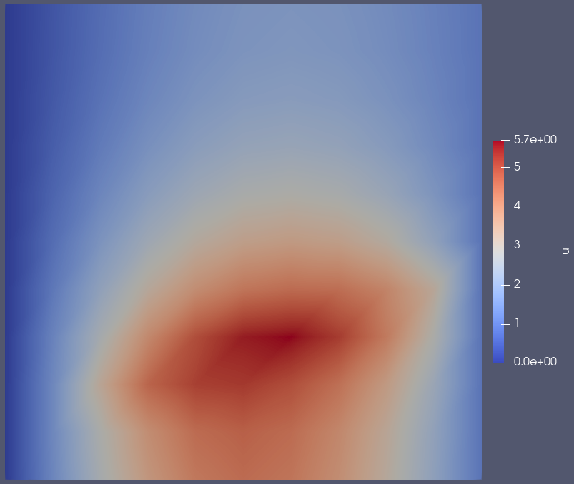
Figure 1: Simple diffusion line source example result.
![The result pictured in [result] with a mesh overlay.](../../../large_media/ray_tracing/simple_diffusion_line_source_mesh.png)
Figure 2: The result pictured in Figure 1 with a mesh overlay.
Just for the purposes of producing a more appealing picture, let's add some adaptivity to the mix to refine the region around the ray.
Take note of the [Adaptivity] block in the input file:
[Adaptivity<<<{"href": "../../../syntax/Adaptivity/index.html"}>>>]
  steps<<<{"description": "The number of adaptive steps to use when doing a Steady simulation."}>>> = 0 # 5
  marker<<<{"description": "The name of the Marker to use to actually adapt the mesh."}>>> = marker
  initial_marker<<<{"description": "The name of the Marker to use to adapt the mesh during initial refinement."}>>> = marker
  max_h_level<<<{"description": "Maximum number of times a single element can be refined. If 0 then infinite."}>>> = 5
  [Indicators<<<{"href": "../../../syntax/Adaptivity/Indicators/index.html"}>>>/indicator]
    type = GradientJumpIndicator<<<{"description": "Compute the jump of the solution gradient across element boundaries.", "href": "../../../source/indicators/GradientJumpIndicator.html"}>>>
    variable<<<{"description": "The name of the variable that this side indicator applies to"}>>> = u
  []
  [Markers<<<{"href": "../../../syntax/Adaptivity/Markers/index.html"}>>>/marker]
    type = ErrorFractionMarker<<<{"description": "Marks elements for refinement or coarsening based on the fraction of the min/max error from the supplied indicator.", "href": "../../../source/markers/ErrorFractionMarker.html"}>>>
    indicator<<<{"description": "The name of the Indicator that this Marker uses."}>>> = indicator
    coarsen<<<{"description": "Elements within this percentage of the min error will be coarsened.  Must be between 0 and 1!"}>>> = 0.1
    refine<<<{"description": "Elements within this percentage of the max error will be refined.  Must be between 0 and 1!"}>>> = 0.5
  []
[]Setting the number of adaptivity steps to 5 via a command line argument, i.e.:
./ray_tracing-opt -i test/tests/raykernels/line_source_ray_kernel/simple_diffusion_line_source.i Adaptivity/steps=5
leads to the well-refined and visually satisfying result below in Figure 3.

Figure 3: Simple diffusion line source example result with adaptivity.
![The result pictured in [result-adaptivity] with a mesh overlay.](../../../large_media/ray_tracing/simple_diffusion_line_source_adaptivity_mesh.png)
Figure 4: The result pictured in Figure 3 with a mesh overlay.