Step 5: Energy Curve
The input file for this step can be found here: s5_energycurve.i
Input File
We are going to make two more changes and our simulation will be complete. First, since we noticed that the variable residuals did not match, we will scale one of the variables to get a better match. Second, we will calculate the total energy of the surface and output it so that we can check if it has an S-curve shape.
Scaling
[Variables]
  [c]   # Mole fraction of Cr (unitless)
    order = FIRST
    family = LAGRANGE
    scaling = 1e+04
  []
  [w]   # Chemical potential (eV/mol)
    order = FIRST
    family = LAGRANGE
  []
[]
If you wish you can remove the debug block, or you can keep it to check that the scaling is correct.
Free energy curve
Remember our Cahn Hilliard equation:
Energy comes from both the free energy density function term and the gradient energy curve. We need to combine these in order to calculate the total energy of the surface. To do this we will define an auxiliary variable, and use a built-in auxiliary kernel to combine the terms. We will output the variable to the Exodus file, and the integral of the variable to the csv file.
[AuxVariables]
  [f_density]   # Local energy density (eV/mol)
    order = CONSTANT
    family = MONOMIAL
  []
[]

[AuxKernels]
  # Calculates the energy density by combining the local and gradient energies
  [f_density]   # (eV/mol/nm^2)
    type = TotalFreeEnergy
    variable = f_density
    f_name = 'f_loc'
    kappa_names = 'kappa_c'
    interfacial_vars = c
  []
[]
The auxiliary variable f_density returns the total energy density at each point on the surface. In order to get the total free energy, we have to integrate the variable in a Postprocessor.
  [total_energy]          # Total free energy at each timestep
    type = ElementIntegralVariablePostprocessor
    variable = f_density
  []
If you wish you may remove any of the Postprocessors that you feel are unnecessary for the simulation at this point, or you may continue trying to optimize the simulation by changing values in the Preconditioning and Executioner blocks.
Results

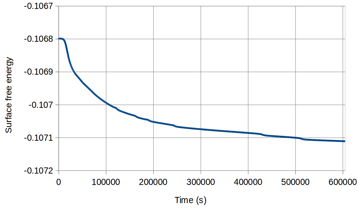
Surface free energy curve
The surface results should look the same as the last simulation. What we really want to look at is what the surface energy looks like throughout the simulation. The plot of the total energy is to the right. Note that the post-processor values are not calculated at the initial condition, so to replicate this plot you must remove that value from the csv file.
From the plot we can see that the energy plot does have the S-curve shape we expected. We have verified that all of our expectations for how the system behaves are correct and therefore we can assume that our model is working correctly.