Flashlight Point Sources
A "flashlight" point source is an anisotropic point source that emits in a cone about a direction . The cone is defined by the vector along the cone axis and half of the opening angle in degrees.
The Ray Tracing Module is utilized for this example to discretize the angular integration. An angular quadrature is sampled within the cone and a Ray generated for each direction. These Rays contribute to PDEs solved on the domain via line sources.
Example
Consider a problem on a two-dimensional mesh in the physical domain . It will contain a reaction term formed by the Reaction / ADReaction kernel and a diffusion term formed by the Diffusion kernel. The anisotropic point source located at emits a source in a cone about . The right boundary will specularly reflect the point source.
The input begins with the basic definition (the mesh, the Reaction / ADReaction and Diffusion kernels, and an Executioner System) as:
[Mesh<<<{"href": "../../../syntax/Mesh/index.html"}>>>]
  [gmg]
    type = GeneratedMeshGenerator<<<{"description": "Create a line, square, or cube mesh with uniformly spaced or biased elements.", "href": "../../../source/meshgenerators/GeneratedMeshGenerator.html"}>>>
    dim<<<{"description": "The dimension of the mesh to be generated"}>>> = 2
    nx<<<{"description": "Number of elements in the X direction"}>>> = 10
    ny<<<{"description": "Number of elements in the Y direction"}>>> = 10
    xmax<<<{"description": "Upper X Coordinate of the generated mesh"}>>> = 5
    ymax<<<{"description": "Upper Y Coordinate of the generated mesh"}>>> = 5
  []
[]

[Variables<<<{"href": "../../../syntax/Variables/index.html"}>>>/u]
[]

[Kernels<<<{"href": "../../../syntax/Kernels/index.html"}>>>]
  [reaction]
    type = Reaction<<<{"description": "Implements a simple consuming reaction term with weak form $(\\psi_i, \\lambda u_h)$.", "href": "../../../source/kernels/Reaction.html"}>>>
    variable<<<{"description": "The name of the variable that this residual object operates on"}>>> = u
  []
  [diffusion]
    type = Diffusion<<<{"description": "The Laplacian operator ($-\\nabla \\cdot \\nabla u$), with the weak form of $(\\nabla \\phi_i, \\nabla u_h)$.", "href": "../../../source/kernels/Diffusion.html"}>>>
    variable<<<{"description": "The name of the variable that this residual object operates on"}>>> = u
  []
[]

[Executioner<<<{"href": "../../../syntax/Executioner/index.html"}>>>]
  type = Steady
  solve_type = PJFNK
  petsc_options_iname = '-pc_type -pc_hypre_type'
  petsc_options_value = 'hypre boomeramg'
[]Defining the Study
A ConeRayStudy is defined that generates and executes the rays within the cone:
[UserObjects<<<{"href": "../../../syntax/UserObjects/index.html"}>>>/study]
  type = ConeRayStudy<<<{"description": "Ray study that spawns Rays in the direction of a cone from a given set of starting points.", "href": "../../../source/userobjects/ConeRayStudy.html"}>>>

  start_points<<<{"description": "The point(s) of the cone(s)."}>>> = '1 1.5 0'
  directions<<<{"description": "The direction(s) of the cone(s) (points down the center of each cone)."}>>> = '2 1 0'
  half_cone_angles<<<{"description": "Angle of the half-cones in degrees (must be <= 90)"}>>> = 2.5
  ray_data_name<<<{"description": "The name of the Ray data that the angular quadrature weights and factors will be filled into for properly weighting the line source per Ray."}>>> = weight

  # Must be set with RayKernels that
  # contribute to the residual
  execute_on<<<{"description": "The list of flag(s) indicating when this object should be executed. For a description of each flag, see https://mooseframework.inl.gov/source/interfaces/SetupInterface.html."}>>> = PRE_KERNELS

  # For outputting Rays
  always_cache_traces<<<{"description": "Whether or not to cache the Ray traces on every execution, primarily for use in output. Warning: this can get expensive very quick with a large number of rays!"}>>> = true
[]A summary of the set parameters is as follows:
"start_points" - The apex of the cone, defined as
"directions" - The direction of the center line of the cone, defined as .
"half_cone_angles" - Half of the opening angle of the cone in degrees, defined as
"ray_data_name" - A name for the data on the Ray to be registered that stores the weight from the angular quadrature
"execute_on" - Set to
PRE_KERNELSso that the Rays are executed with the residual evaluation"always_cache_traces" - Enabled to cache information for outputting the Rays in a mesh form (see RayTracingMeshOutput)
Defining the RayBCs
RayBCs are objects that operate on Rays that intersect a boundary. We require the following:
A RayBC that reflects the rays on the right boundary in a specular manner
A RayBC that ends the rays on the top boundary that are reflected off of the right boundary
In specific, we will add a ReflectRayBC on the right boundary and a KillRayBC on the top boundary. These are implemented as follows:
[RayBCs<<<{"href": "../../../syntax/RayBCs/index.html"}>>>]
  [reflect]
    type = ReflectRayBC<<<{"description": "A RayBC that reflects a Ray in a specular manner on a boundary.", "href": "../../../source/raybcs/ReflectRayBC.html"}>>>
    boundary<<<{"description": "The list of boundary IDs from the mesh where this object applies"}>>> = 'right'
  []
  [kill_rest]
    type = KillRayBC<<<{"description": "A RayBC that kills a Ray on a boundary.", "href": "../../../source/raybcs/KillRayBC.html"}>>>
    boundary<<<{"description": "The list of boundary IDs from the mesh where this object applies"}>>> = 'top'
  []
[]At this point, it is important to note that it is not necessary to provide the "rays" parameter to any added RayKernels or RayBCs, unlike what was done in Using Line Sources or Computing Line Integrals. This is because the ConeRayStudy does not have Ray registration enabled (see Ray Registration for more information). Ray registration requires that a name be associated with each Ray. It is disabled in the ConeRayStudy because the large number of Rays generated makes it unreasonable to name each one.
Defining the RayKernel
RayKernels are objects that are executed on the segments of the Rays. In this case, each Ray will act as a line source as it is traced. For this, we will add a LineSourceRayKernel as follows:
[RayKernels<<<{"href": "../../../syntax/RayKernels/index.html"}>>>/line_source]
  type = LineSourceRayKernel<<<{"description": "Demonstrates the multiple ways that scalar values can be introduced into RayKernels, e.g. (controllable) constants, functions, postprocessors, and data on rays. Implements the weak form $(\\psi_i, -f)$ along a line.", "href": "../../../source/raykernels/LineSourceRayKernel.html"}>>>
  variable<<<{"description": "The name of the variable that this RayKernel operates on"}>>> = u

  # Scale by the weights in the ConeRayStudy
  ray_data_factor_names<<<{"description": "The names of the Ray data to scale the source by (if any)"}>>> = weight
[]Take note of the supplied parameter "ray_data_factor_names". Recall that within the defined ConeRayStudy, we supplied the parameter "ray_data_name", which is the Ray data that will store the weights from the angular quadrature and the user defined scaling factors (if any). The "ray_data_factor_names" parameter in LineSourceRayKernel will scale the source by the given Ray data, which effectively scales the line source term by the angular quadrature weights and the user defined scaling factors (if any).
Result
The problem is ran with
./ray_tracing-opt -i test/tests/userobjects/cone_ray_study.i
and the result (in cone_ray_study_out.e) is pictured below in Figure 1.
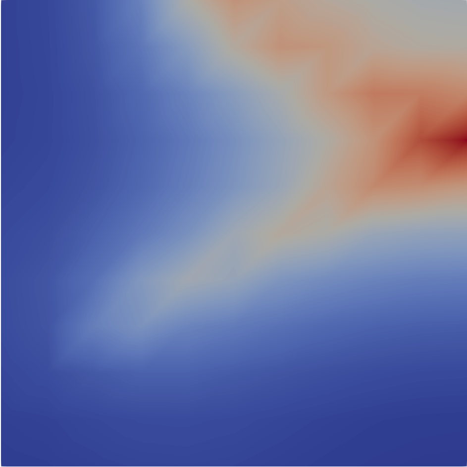
Figure 1: Result for the diffusion-reaction problem with a flashlight point source.
Refined Result
Admittedly, the result in Figure 1 is not particularly satisfying in a visual sense. We need more elements! Let's take advantage of the Adaptivity System. With this, take note of the Adaptivity block:
[Adaptivity<<<{"href": "../../../syntax/Adaptivity/index.html"}>>>]
  steps<<<{"description": "The number of adaptive steps to use when doing a Steady simulation."}>>> = 0 # 6 for pretty pictures
  marker<<<{"description": "The name of the Marker to use to actually adapt the mesh."}>>> = marker
  initial_marker<<<{"description": "The name of the Marker to use to adapt the mesh during initial refinement."}>>> = marker
  max_h_level<<<{"description": "Maximum number of times a single element can be refined. If 0 then infinite."}>>> = 6
  [Indicators<<<{"href": "../../../syntax/Adaptivity/Indicators/index.html"}>>>/indicator]
    type = GradientJumpIndicator<<<{"description": "Compute the jump of the solution gradient across element boundaries.", "href": "../../../source/indicators/GradientJumpIndicator.html"}>>>
    variable<<<{"description": "The name of the variable that this side indicator applies to"}>>> = u
  []
  [Markers<<<{"href": "../../../syntax/Adaptivity/Markers/index.html"}>>>/marker]
    type = ErrorFractionMarker<<<{"description": "Marks elements for refinement or coarsening based on the fraction of the min/max error from the supplied indicator.", "href": "../../../source/markers/ErrorFractionMarker.html"}>>>
    indicator<<<{"description": "The name of the Indicator that this Marker uses."}>>> = indicator
    coarsen<<<{"description": "Elements within this percentage of the min error will be coarsened.  Must be between 0 and 1!"}>>> = 0.25
    refine<<<{"description": "Elements within this percentage of the max error will be refined.  Must be between 0 and 1!"}>>> = 0.5
  []
[]As in the input, the number of adaptivity steps is currently set to 0. We will set that to 6 via a command line argument and run again with:
mpiexec -n 4 ./ray_tracing-opt -i test/tests/userobjects/cone_ray_study.i Adaptivity/steps=6

Figure 3: Refined result for the diffusion-reaction problem with a flashlight point source.
![The result pictured in [adaptivity] with a mesh overlay.](../../../large_media/ray_tracing/cone_ray_study_u_mesh.png)
Figure 4: The result pictured in Figure 3 with a mesh overlay.
Result with Ray Overlay
For a little more pretty-picture goodness, we will also output the generated Rays using RayTracingMeshOutput.
Recall the "always_cache_traces" parameter that was set to true for the ConeRayStudy. This was enabled so that the trace information could be cached for use in output. Take note of the Output block with the RayTracingExodus object:
[Outputs<<<{"href": "../../../syntax/Outputs/index.html"}>>>]
  exodus<<<{"description": "Output the results using the default settings for Exodus output."}>>> = true

  [rays]
    type = RayTracingExodus<<<{"description": "Outputs ray segments and data as segments using the Exodus format.", "href": "../../../source/outputs/RayTracingExodus.html"}>>>
    study<<<{"description": "The RayTracingStudy to get the segments from"}>>> = study
    execute_on<<<{"description": "The list of flag(s) indicating when this object should be executed. For a description of each flag, see https://mooseframework.inl.gov/source/interfaces/SetupInterface.html."}>>> = FINAL
  []
[]The output file cone_ray_study_rays.e is also generated with the simulation. We will overlay this mesh on top of the original output with adaptivity to obtain what follows in Figure 2.
![Result for the diffusion-reaction problem with a flashlight point source, with adaptivity, and with a [RayTracingExodus.md] overlay.](../../../large_media/ray_tracing/cone_ray_study_rays.png)
Figure 2: Result for the diffusion-reaction problem with a flashlight point source, with adaptivity, and with a RayTracingExodus overlay.