List of tutorials
All tutorials are written assuming that you are reasonably familiar with MOOSE. If you find most of the tutorials difficult to follow, please refer to the official MOOSE website for learning resources.
Tutorial 14: Random field generation by KL expansion
In this tutorial, we will generate a spatially varied material property field with a controlled correlation length.
The generated field is ready to be used in Tutorial 5.
Step 0: required packages
Boost is required for patch generation. While your Conda MOOSE environment is active, install boost by running:
conda install boost
Step 1: build the Karhunen-Loève expansions
For this step, navigate to folder factorize/.
In klexpansion.C:
Line 52 provided the mesh for the kl expansion construction (this mesh does not have to be identical to the mesh for the physical problem).
MeshTools::Generation::build_square(mesh, 50, 50, 0, 100, 0, 100, QUAD4);
builds a 2d square mesh occupying coordinate [0,100]x[0,100], and discretizing by 50x50 QUAD4 elements. This mesh has to be fine enough to fully resolve the correlation length. You need at least 4 nodes per correlation length.
Guides on generating other types of meshes MeshTools:Generation
Can also read in a mesh by mesh.read("YourMesh");
Line 207-208:
  PSE covariance_x(10, 100);
  PSE covariance_y(10, 100);
defines the kernel type (PSE or PE), correlation length (or any value given by the user), and periodicity (the size of the domain). Kernels are defined in covariance_functions.h
To compile this code
make
#  To clean old output and runtime files, run make clean
After a successful compilation, run the executable by
./klexpansion-opt
or in parallel, by
mpiexec -n NumberofTasks ./klexpansion-opt
Once it is complete, the KL expansions needed for random field sampling will be stored in a new exodus file. By default this is basis.e.
Step 2: sampling the random field
For this step, navigate to sample/
In code sample.C:
Line 47
mesh.read("../factorize/basis.e");
reads the KL expansions generated in step 1. Update this line as needed, and keep line 53 reading the same mesh as line 47.
Line 78-80:
  std::vector<Real> Gc; # the name of field  1
  std::vector<Real> psic; # the name of field  2
  compute_correlated_Gamma_fields(Xi_1, Xi_2, Gc, 8e-4, 0.03, psic, 3e-5, 0.03, 0);
Field will be generated with mean and coefficient of variation . Field will be generated with mean and COV . The correlation between the two fields is .
To compile the code
make
To sample a random field
./sample-opt
The tutorial code generates a new field with the default name fields.e.
Each time you run ./sample-opt, a different field is generated with an updated random seed.
Example fields
Below is a set of example random fields generated using different kernels, correlation lengths, and geometries.
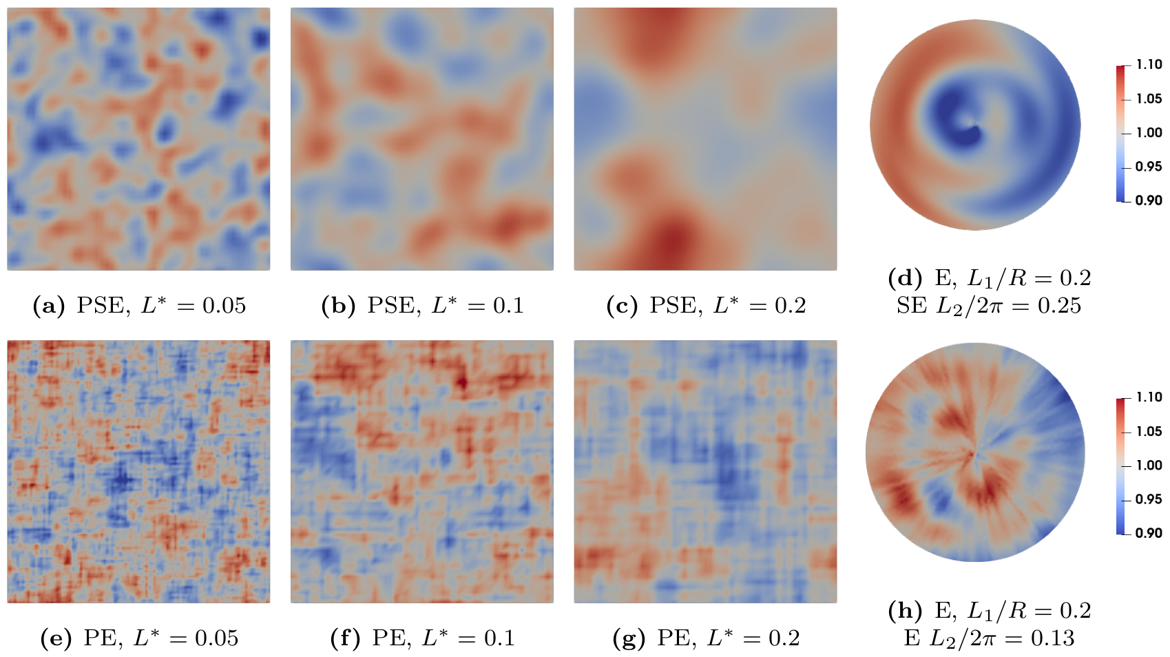
Figure 1: Samples of the (non-Gaussian) random field, generated with mean and coefficient of variation set to 1.0 and 3\%, respectively, for the sake of illustration. Here, is the normalized correlation length on the rectangular domain. Zeng et al. (2025)
Related source code
References
- Bo Zeng, Johann Guilleminot, and John E. Dolbow.
Examining crack nucleation under spatially uniform stress states with a complete phase-field model for fracture.
Theoretical and Applied Fracture Mechanics, pages 105170, 2025.
URL: https://www.sciencedirect.com/science/article/pii/S0167844225003283, doi:https://doi.org/10.1016/j.tafmec.2025.105170.[BibTeX]